Discrete Diffusion Processes

Introduction

Diffusion is often discussed in reference to the continous case that uses a normal distribution to model a complex data distribution. The continous case works well when the Markov Decision Process (MDP) of a problem is continous in nature e.g images. It is less suitable when the MDP is discrete e.g graphs, text. For such an MDP a discrete distribution is preferrable and better suited for the noise distribution. However adapting discrete noise to the diffusion framework is not trivial.

While the discrete process shares some similarities with its continuous counterpart, there are quite some differences with regards to the reverse process and training objective. In my opinion, some of the differences - noise distribution and training objective - shed some insights into the nature of diffusion processes. In this post, I’ll discuss the discrete case and aspects of it that can be generalized to the continous case.

Background

In diffusion we want to learn a reverse transition from a random state to a desired state. A state refers to a configuration of features that make up a datapoint and a desired state is a datapoint from the data distribution that we want to model. The collection of all possible feature configurations makes up the state space and any random configuration within it refers to a random state.

The features in the discrete case take on one of K discrete values.

$\textbf{x}_{t} = [x_{0}, x_{1}, ..., x_{D}], \quad x_{d} \in \{0, K\}$

Sometimes we may prefer to represent them as a collection of one-hot vectors

$\textbf{x}_{t} = [x_{0}, x_{1}, ..., x_{D}], \quad x_{d} \equiv e_{i} \in \{0, 1\}^{K}$

To transition into another state, we sample from a categorical distribution whose success probabilities or mean parameter is the product of the current state and a transition matrix

$\begin{aligned} q(\textbf{x}_{t+1}|\textbf{x}_{t}) = \text{Cat}(\textbf{x}_{t+1}; \textbf{z}_{t+1} = \textbf{x}_{t}Q_{t+1}^{\top})\\ \end{aligned}$

The original diffusion paper by Sohl-Dickstein et al used a Bernoulli distribution for the discrete binary case and subsequent papers have used the Categorical distribution as an extension to three or more discrete values.

Transition Matrix

The transition matrix is a K-by-K matrix that gives the probability of a feature, with a given value, taking on another value in the next timestep. There are different transition matrices proposed by Austin et al but the most straightforward is the uniform diffusion matrix whose elements can be expressed as

$Q_{ij}(t) = \begin{cases} (1 - \beta_{t}) + \beta_{t}/K &\quad i = j\\ \beta_{t}/K &\quad i \neq j\\ \end{cases}$

where beta is the current diffusion rate. The matrix form can be expressed as

$Q_{t} = \alpha_{t}\mathbb{I}_{k} + (1 - \bar{\alpha}_{t})/K, \quad \alpha_{t} = (1 - \beta_{t})$

After many diffustion timesteps, we can represent the cumulative transition matrix as

$\bar{Q}_{t} = \bar{\alpha}_{t}\mathbb{I}_{k} + (1 - \bar{\alpha}_{t})/K, \quad \bar{\alpha}_{T} = \prod_{t=0}^{T}\alpha_{t}$

For a sufficient number of timesteps, this matrix is equivalent to the cumulative product of all the transition matrices at prior timesteps

$\bar{Q}_{T} \equiv Q_{1}\prod_{t=2}^{T}Q_{t}^{\top}$

At such point, the alpha term becomes negligible and the cumulative transition matrix enters a stationary distribution in which there is a uniform probability of a feature taking any of the K discrete values. This ergodic property of the transition matrix mirrors that of the continous case where the standard deviation of the Gaussian noise remains unchanged after multiple timesteps.

We can thus represent the forward process as

$q(\textbf{x}_{t}|\textbf{x}_{0}) = \text{Cat}(\textbf{x}_{t}; \textbf{z}_{t}), \quad \textbf{z}_{t} = \textbf{x}_{0}\bar{Q}_{t}^{\top} = \textbf{x}_{0}\prod^{t}_{i=1}Q_{i}$

Reverse Process

Similar to the typical diffusion process, we cannot determine the reverse transition probability without knowledge of the initial state. Here we also apply Bayes rule to get this probability

$q(\textbf{x}_{t-1}|\textbf{x}_{t}, \textbf{x}_{0}) = \frac{q(\textbf{x}_{t}|\textbf{x}_{t-1}, \textbf{x}_{0})q(\textbf{x}_{t-1}|\textbf{x}_{0})}{q(\textbf{x}_{t}|\textbf{x}_{0})}$

since we know the value of a feature in the current and inital states, we can express the probability as

$\begin{aligned} q(\textbf{x}_{t-1}|x_{t}=k, x_{0}=l) &= \frac{q(x_{t}=k|\textbf{x}_{t-1}, x_{0}=l)q(\textbf{x}_{t-1}|x_{0} = l)}{q(x_{t} = k|x_{0} = l)} \\ &= \frac{q(x_{t}=k|\textbf{x}_{t-1}, x_{0}=l)q(\textbf{x}_{t-1}|x_{0} = l)}{\sum_{\textbf{x}_{t-1}}q(x_{t}=k|\textbf{x}_{t-1}, x_{0}=l)q(\textbf{x}_{t-1}|x_{0} = l)} \end{aligned}$

Let’s discuss each of the probability terms above. The likelihood depends on the prior state and value of the initial state. The initial state however is redundant in this case because the value of the current state only depends on that of the prior state. Although the prior state is unobserved, we can still get the probability of going to the current state value by multiplying the one-hot vector for a feature in said state with the transition matrix. This will give the probability of going from any value in the prior state to that of the current state

$q(x_{t}=k|\textbf{x}_{t-1}, x_{0}=l) = q(x_{t}=k|\textbf{x}_{t-1}) = e_{k}Q_{t}^{\top}$

Next is the prior probability which is straightforward because it is simply running the forward process from the initial state value to the prior state. This is simply

$q(\textbf{x}_{t-1}|x_{0}=l) = e_{l}\bar{Q}_{t-1}$

Finally we have the marginal which can be expressed as a sum of the numerator over all K values or it can be accessed from the current cumulative transition matrix. Note that

$\sum_{i, j} \bar{Q}_{i}(t-1) \odot Q_{j}(t)^{\top} = \bar{Q}_{t-1}Q_{t}^{\top} \equiv \bar{Q}_{t}$

Each cell of the resulting matrix is the sum of the cartesian product between the rows of the prior cumulative matrix and columns of the current transition matrix. Therefore the product of this matrix and the one-hot vectors for both the initial and current states returns the sum at the corresponding indices.

Hence the reverse process can be computed as

$\begin{aligned} q(\textbf{x}_{t-1}|x_{t}=k, x_{0}=l) = \text{Cat}(\textbf{x}_{t-1}; \textbf{z}_{t-1}), \quad \textbf{z}_{t-1} &= \frac{Q_{t}e_{k}^{\top} \odot \bar{Q}_{t-1}e_{l}^{\top}}{\sum Q_{t}e_{k}^{\top} \odot \bar{Q}_{t-1}e_{l}^{\top}}\\ &= \frac{Q_{t}e_{k}^{\top} \odot \bar{Q}_{t-1}e_{l}^{\top}}{e_{k}\bar{Q}_{t}e_{l}^{\top}} \end{aligned}$

Training Objective

The discrete model is trained using the typical diffusion objective function

$\mathbb{KL}(q(\textbf{x}_{T}|\textbf{x}_{0})||p_{\theta}(\textbf{x}_{0})) + \sum^{T}_{t=2}\mathbb{KL}(q(\textbf{x}_{t-1}|\textbf{x}_{t}, \textbf{x}_{0})\|p_{\theta}(\textbf{x}_{t-1}|\textbf{x}_{t})) - p_{\theta}(\textbf{x}_{0}|\textbf{x}_{1})$

where, for the most part, we minimize the KL divergence between the reverse and the learned transition probabilities across the diffusion trajectories

$\mathbb{E}_{q(\textbf{x}_{t-1}|\textbf{x}_{t}, \textbf{x}_{0})}[\text{log } q(\textbf{x}_{t-1}|\textbf{x}_{t}, \textbf{x}_{0}) - \text{ log } p_{\theta}(\textbf{x}_{t-1}|\textbf{x}_{t})]$

The learned reverse transition uses a neural network to predict the initial state during training so that at test time its prediction can also be used to generate the next state in the reverse process. To train the model, we can simply minimize the cross entropy of the network which is the usual multi-class learning objective w.r.t the value of each feature in the initial state

$\underset{\theta}{\text{argmin }} \mathbb{E}[\text{log } p_{\theta}(\textbf{x}_{0}|\textbf{x}_{t})]$

The cross entropy objective also minimizes the KL divergence term above, because the learned reverse probability can be expressed as the sum of the reverse probability for each discrete value of the initial state and the network’s probability of said value

$p_{\theta}(\textbf{x}_{t-1}|\textbf{x}_{t}) = \sum_{\textbf{x}_{0}} q(\textbf{x}_{t-1}|\textbf{x}_{t}, \textbf{x}_{0})p_{\theta}(\textbf{x}_{0}|\textbf{x}_{t})$

At the objective minimum, the network places most of the probability mass on the value of the initial state such that the probability of other discrete values is zero. Then both the learned and reverse probabilities are equal and the divergence is also minimized.

Example

As an example, I’ll generate the Zachary’s Karate Club graph using discrete diffusion. The Zachary Karate Club is a frequently used graph representation task. The graph models the social interactions of 34 Karate Club members who are split into two groups at some point during their interaction.

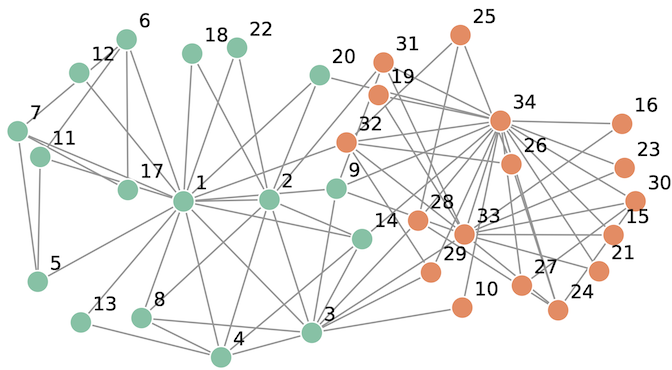
The edges and nodes of this graph will be modeled separately. Each edge represents social interaction between a pair of members, so for members that didn’t interact there is no edge. Therefore all possible edges in the graph take on a binary value indicating the interaction between members. Since members are split into two groups, each node also take on a binary value indicating the group they eventually belonged to.

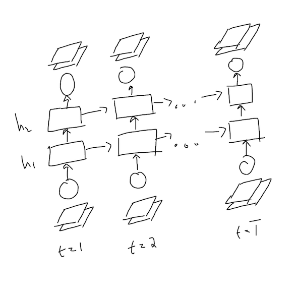
To model both the edges and nodes, I used a recurrent neural network (RNN) with the given number of diffusion timesteps. The network has 2 hidden layers of 128 units each. Its input is a batch of sampled diffusion states and its output is the predicted initial state. A state is a vector containing the value of all the nodes or edges. For the diffusion model I used 360 timesteps, a variance or diffusion schedule of $(0.001, 0.05)$ and 20 training epoches.

The sample below is the reverse process generation of the Karate graph from a random graph.

Conclusion

Discrete diffusion is an interesting extension of the original diffusion framework to problems that involve discrete spaces. Since there are many of such problems, active areas of research include molecular generation and large language models etc. In later posts, I hope to discuss some of these areas in detail but until then ciao!