Diffusion Processes

Introduction

Last year’s International Conference on Machine Learning (ICML) in Vancouver, BC was my first conference in three years and at the conference there were a lot of interesting papers related to diffusion processes. Prior to the conference, I wasn’t following the field but since then I’ve taken a liking to it and so in this post, I’ll briefly outline what a diffusion model is, its component processes and model training.

What is Diffusion?

Diffusion is a generative modelling technique that generates data from random noise within a finite series of steps. It entails transforming data into random noise and then learning the reverse transformation in order to regenerate the data. The noise transformation process is referred to as the forward process while the generation process is referred to as the reverse process.

Forward Process

The forward diffusion process transforms data into random noise. However instead of doing this in a single or a few steps, it is done over many timesteps by perturbing the data with a small amount of zero-mean Gaussian noise. Locally, between any pair of consecutive timesteps, there is little difference in the data but globally, across multiple timesteps, the data is noisy.

We can express the transformation between adjacent timesteps as

$x_{t} = \sqrt{1 - \beta_{t}}x_{t-1} + \sqrt{\beta_{t}}\epsilon_{t-1} \text{ ,} \quad \epsilon_{t-1} \sim \mathcal{N}(0, 1)$

where beta is the variance parameter that controls the amount of noise or rate of diffusion at a particular timestep. Initially we start off with a very small rate but steadily increase it at each timestep such that

$\beta_{1} < \beta_{2} < ... < \beta_{T}$

Starting from the initial data, we can express the data at any given time in the forward process as

$x_{t} = \sqrt{\bar{\alpha}_{t}}x_{0} + \sqrt{1 - \bar{\alpha}_{t}}\epsilon_{t-1} \text{ ,} \quad \bar{\alpha}_{t} = \prod^{t}_{i=1}{\alpha_{i}} = \prod^{t}_{i=1}{(1 - \beta_{i})}$

This weighted additive noise process can also be seen as sampling the data from a Gaussian distribution that is conditioned on the initial data

$q(x_{t}|x_{0}) = \mathcal{N}(x_{t}; \sqrt{\bar{\alpha}_{t}}x_{0}, (1 - \bar{\alpha})_{t})$

To facilitate learning, we run the forward process for a given data over many iterations and then use the data at each timestep to train the diffusion model in the reverse process.

Reverse Process

As it suggests, in the reverse process the diffusion model learns to remove noise that was added during the forward process. Unlike the forward process where the data is sequential, in the reverse process it is identical and independent. This lack of prior information however makes denoising the data at any timestep infeasible.

The task becomes feasible if we include information about the intial data. Doing so we can sample the denoised image from the following posterior distribution

$\text{q}(x_{t-1}|x_{t}, x_{0}) = \mathcal{N}(x_{t-1}; \tilde{\mu}(x_{t}, x_{0}), \tilde{\beta}_{t}\mathbf{I})$

where

$\tilde{\mu}(x_{t}, x_{0}) = \frac{\sqrt{\alpha_{t}}(1 - \bar{\alpha}_{t-1})}{(1 - \bar{\alpha}_{t})}x_{t} + \frac{\sqrt{\bar{\alpha}_{t - 1}}(1 - \alpha_{t})}{(1 - \bar{\alpha}_{t})}x_{0}$

and

$\tilde{\beta}_{t} = \frac{1 - \bar{\alpha}_{t-1}}{1 - \bar{\alpha}_{t}}\beta_{t}$

Although the initial data is available during training, it is unavailable during testing. To denoise the current data, we use an approximation to the initial data that is learned during training. This learned approximation can come from a neural network. The network can be seen as a denoising auto-encoder as it attempts to generate the original data from its noisy versions. This works pretty well and generates true samples of the data distribution rather than just the mean of the distribution.

The denoising diffusioin model by [] goes one step further. It reformulates the posterior mean above in terms of the current data and noise added. Rather than estimate the initial data, it estimates the noise itself and removes it from the current data. This is a lot harder to do as it requires more powerful neural network architectures that are able to capture the noise.

Training Objective

Diffusion models optimize the Evidence Lower Bound (ELBO) objective

$\begin{aligned} \text{log }p_{\theta}(x_{0}) \geq \text{log }p_{\theta}(x_{0}) - \mathbb{KL}(q(x_{1:T}|x_{0})\|p_{\theta}(x_{1:T}|x_{0})) \end{aligned}$

To maximize this lower bound, we can express the Kubler-Libler divergence as

$\mathbb{KL}(q(x_{T}|x_{0})||p_{\theta}(x_{0})) + \sum^{T}_{t=2}\mathbb{KL}(q(x_{t-1}|x_{t}, x_{0})\|p_{\theta}(x_{t-1}|x_{t})) - p_{\theta}(x_{0}|x_{1})$

where we have a divergence between the reverse probability and the learned probability across the diffusion timesteps. Since we have the analytical form of the reverse probability, this KL divergence reduces to a squared loss regression between the mean of learned probability and that of the reverse probability

$\underset{\theta}{\text{min }} \|\tilde{\mu}(x_{t}, x_{0}) - \mu_{\theta}(x_{t})\|^{2}$

Depending on how we choose to parameterize the mean, either as the initial data or noise, we end up with two different objective functions where the target is the initial data or current noise from the forward process and the regressor is the network output.

Examples

To illustrate the capability of diffusion models, we can use two relatively simple datasets: Swiss Roll and the MNIST dataset. In both examples, the diffusion model learns to predict the initial data during training and uses an approximation of this data to generate the samples shown.

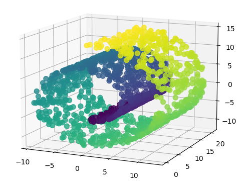
Swiss Roll

The SwissRoll dataset is a well known dataset for dimensional embedding. It consists of points that form a 3D swiss roll with different color gradients. For our example, we simply take the 2 dimensions that best illustrate the swiss roll structure as shown below

For this dataset, the network is a MultiLayer Perceptron (MLP) with a radial basis function hidden layer and 2 separate linear outputs. I used a variance between 0.001 and 0.05 for 40 diffusion steps. The model was trained with 100 points per batch for 1500 epochs. The image below illustrates the reverse process for a few sampled digits

MNIST

The MNIST dataset is a popular machine learning image dataset comprising of 28 x 28 greyscaled handwritten digits numbered 0 to 9.

For this dataset, the network used is a U-Net with ShuffleNet units and a multilayer perceptron (MLP) for embedding each timestep. There were 1000 diffusion timesteps with a variance between 0.0001 and 0.02. The model was trained for 10 epochs with a batch size of 128. The image below illustrates the reverse process for a few sampled digits

Conclusion